Pay It Forward Train
November 29, 2020 was a terrible day. In need of some caffeine, I pulled into McDonald's and ordered a single black coffee. At the window the cashier refused my credit card. You see, there was a "Pay it Forward Train" going on and my order was already paid for. I was then posed the fateful question, "Would you like to pay for the person behind you?"
In a dazed state I inquired how much the next order was; after all I was only planning to spend less than $2. It was $45! Now I can be a bit of curmudgeon, but the idea of paying $45 to receive a coffee should be absurd to anyone. Worse, I couldn't even pay for my own order since the ticket was already closed. A true tragedy.
Sure, the person in front had charitably paid for me, but that wasn't kindness. It was chaos that left me deciding between paying $45 for a coffee or being the jerk who ended the train. I cursed the person who started this ridiculous concept and stole the light from the cashier's eyes as I ended her one ray of joy on an otherwise dreary Sunday morning.
A PiFT is just a lottery to see how much your food costs, and we all know the lottery is a fool's errands. Could this lottery be different? After all, there isn't a house setting odds. Can we build a model and discover an untapped arbitrage opportunity? At the very least, we should be able to set our expectations and be prepared in case we find ourselves in the abomination known as a "Pay it Forward Train".
The Approach
First we need some data. I'm writing a dumb blog in between work, family, and way too many hobbies. I'm not going to travel the country and ask to audit the order history of every PiFT I catch wind of. While I have seen some news articles basking in the idiotic warm and fuzzy feeling that most people associate with this ordeal, they never include any data.
So I'm just going to make it up.
However, we can use some logic and intuition when we create our dummy data. After all, we're testing plausible scenarios. We need to understand the core concepts and drivers of what we're trying to capture in our fake data. The Whataburger example in the link above, stated that their train included 105 customers. While I want to personally shake the hand of the individual brave enough to finally end that madness, let's make our example even bigger, 150 cars.
Since we're also modeling cars not customers, we need to account for the variance in number of passengers. It could be a single, maligned individual like myself or it could be a packed-out minivan trying to swindle hard-earned cash from the car in front of them. These are the uncertain horrors we face.
We also need some menu items to choose from. I made a quick table of 13 popular McDonald's items across a few categories of orders and pulled prices from an online delivery app. Close enough.
| Order Item | Category | Price |
|---|---|---|
| McFlurry | Desert | $4.62 |
| Apple Pie | Desert | $2.06 |
| Black Coffee | Drink | $1.89 |
| Diet Coke | Drink | $1.98 |
| Happy Meal | Meal | $6.32 |
| Big Mac Meal | Meal | $12.56 |
| McCrispy Meal | Meal | $11.69 |
| 10 pc Chicken McNugget Meal | Meal | $12.04 |
| Filet-O-Fish Meal | Meal | $11.69 |
| McChicken | Single | $2.99 |
| Quarter Pounder with Cheese | Single | $6.39 |
| French Fry | Snack | $2.49 |
| 6pc McNuggets | Snack | $3.65 |
This time we'll be using python to make things easier. Showing the code inline is more of a nuisance than a help, but links to download the files will be at the bottom of the page. I'll write a simple script that loops 150 times, each time randomly assigning 1 to 7 passengers and randomly choosing a menu item for each passenger. Do a little data pivoting/charting, and let's take a look at what we have.
Distributions of Order Totals by Passengers
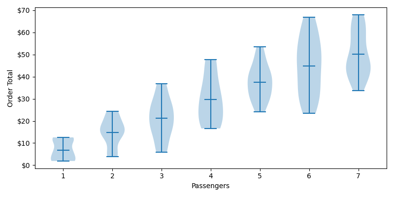
Violin charts are pretty neat. Think of them as bell curves rotated 90 degrees. We can see some obvious trends that we would expect, such as the fact that our median order total is increasing with the number of passengers. We can also see that our distributions tend to get wider as we increase passengers. Intuitively this also makes sense. The menu items are chosen at random, so the number of passengers serves as a multiplier on our variance. The difference between 7 coffees and 7 Big Mac meals is much greater than what a single person could achieve. Lastly, our distributions aren't always normalized, but that's OK for what we're trying to accomplish.
Histogram of Passengers
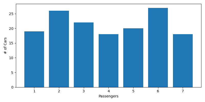
Let's also take a look at a histogram of our cars by passengers. This is pretty evenly distributed, and that's bad. Unless people started catching wind of the train and rounded up all their friends to take advantage of those poor coffee drinkers, we'd expect our histogram to look something like this:
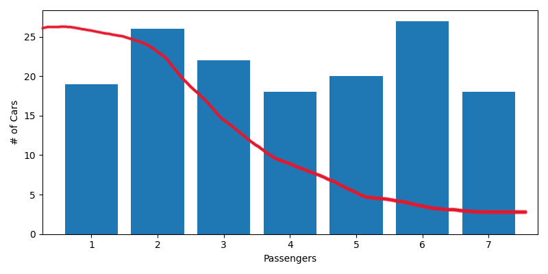
So there are two issues with our fake data so far. Even though it's made up, we want it be realistic. We can easily fix our distribution of passengers by writing a pseudo-random function that weights our passengers more towards the individual. But let's also talk about menu selection. There is likely a lot of correlation between what people order within a car and also with the size of the car. Minivans probably tend to order lots of Happy Meals, and if one person orders a meal then their passenger(s) is more likely to also order a meal rather than a snack. Just like last time, I'm going to ignore that correlation because it's not the interesting part. If that bothers you, you're probably the kind of person that starts Pay it Forward Trains.
Improved Histogram of Passengers
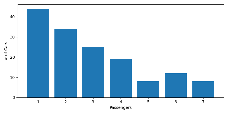
Much better, now our population of 150 cars has way more single passenger cars than packed out minivans. Now of course, this will also change our distributions of order totals. (In fact, every time we simulate a population the data will vary. But that's OK for reasons we'll get into later.)
Improved Distributions of Order Totals by Passengers
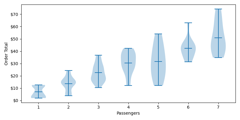
Notice that our distributions aren't as wide with our higher passengers. The passengers still act to multiply our variance, but there just aren't as many cars.
No Such Thing as a Free Lunch
Here's the interesting thing about a PiFT, as a population it is always balanced. Every meal is paid for and the total dollar amount overpaid is equally balanced by the total dollar amount underpaid. However, this is only true for aggregate dollar amounts, not for the individuals, or even the number of individuals. The first person (usually a well-intentioned jerk) always overpays since they pay for their own meal and the person behind them. While the unfortunate, but morally correct, enders of the chain receive their meal for free.
While the first and last person in the train have unique characteristics, everyone within the train is just swapping the price of their orders (Madness!). To make our charts so far we generated a single ordered chain. Let's plot the individual and cumulative effects to analyze in greater detail.
Cumulative History of Over and Under Payment
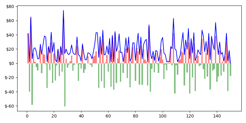
Over payments, where a car pays more in the PiFT than they normally would, are shown in red. Under payments in green. The cumulative over/under payment is shown as the blue line. We can gather a few insights from this chart. The most important is that we always start with an over payment (2 orders) and end with an underpayment (free order). The cumulative line always starts positive and ends at zero. If we imagine some kind of hippie/commie situation where every order in the train was identical, you would have one red bar at the beginning, a cumulative line that stays flat, and a green bar at the end that brings our cumulative bar back down to zero. Our accounts always balance as the train is broken. So later, we'll be dropping the first (villain) and last (hero) data points from our train.
Combining Idiots
Even though the pieces making up this chain are random, and 150 cars seems like a lot, it's nowhere near petty enough. As a single train with one fixed order, each car only faces one scenario. We only end up with a handful of 7-passenger vehicles, and our data could be skewed by pure chance. We need to generate multiple sets of 150 cars, and we need to check multiple orderings within each of those sets. Fortunately, computers make this easier. Even when you write very inefficient python.
How many different ways can these 150 cars be ordered and who is at the front of the train? In the real world, we would interview each of the drivers, check their IQ, and set a inverse probability function where the lower their IQ the more likely they are to start a PiFT. However, we're only looking at the individuals within the train, the ones who are caught up in the madness at no fault of their own. We don't care who starts it.
For any combination of these cars there are 150 options for the idiot conductor. What about the second spot? Well we now only have 149 options, since we've identified the jerk. On and on until we get to the last spot where there is only only option left for our enlightened combo breaker.
We can write it as a product of 150 sequential numbers or just use the factorial notation. Either way we get the same result: $$ Orderings\ of\ Fools = 150 * 149 * 148 * .... * 2 * 1 $$ $$ Orderings\ of\ Fools = 150!$$ $$ Orderings\ of\ Fools = 5.713*10^{262} $$
Considering there are ~1082 atoms in the universe, I don't think I'm simulating that on my laptop. Let's create 10 random groups of 150 cars, and we'll simulate a different ordering of cars for each group 1,000 times. After dropping our conductor and caboose, 1.48 million individual scenarios is much more manageable and still give us very interesting data to work with. Based on our pseudorandom generator, we should expect roughly the following scenarios for each number of passengers:
| Passengers | %age of Population | Scenarios |
|---|---|---|
| 1 | 33% | 488,400 |
| 2 | 25% | 370,000 |
| 3 | 15% | 222,000 |
| 4 | 10% | 148,000 |
| 5 | 8% | 118,400 |
| 6 | 6% | 88,800 |
| 7 | 3% | 44,400 |
The Meat of the Matter
If, like the hero of our story, you find yourself stuck in this predicament, couldn't you merely follow my example? Ask the cashier how much the next order is and then decide?
Sure, if you want to take the easy route like a normal person. Why would we do that when we could make it really complicated and over-prepare us for an extremely rare and ultimately inconsequential situation?
We want to answer two questions on behalf of these underdogs:
- How risky is the PiFT based on number of passengers?
- Is there a defensive order we should make to anticipate a PiFT?
Diving In
Monte Carlo, not just a famous casino in Monaco, but a probabilistic model that is perfect for nondeterministic simulations like the one we just created. Most often used in financial analysis to forecast investment strategies, I can think of no finer application than rationalizing why you should actually hate Pay it Forward Trains.
The gist of how it works is you create a simulation of events that are independent from each other, and you run that simulation over and over. We can then analyze these outcomes to say which events are most likely and the distribution of said events. Monte Carlo is a great way to brute force a problem when you can't/won't calculate.
To give a quick and dirty example, think of a stock that will take one of 5 equally likely steps every year. It can either go up by 3%, 5%, or 10% or down by 6% or 12%. (In reality we often see correlation in stock movement to a previous year in which case we'd be better off treating it as a Markov process, but we'll save that for another time). Let's forecast what will happen over 10 years.
We can quickly determine our extremes, the data points which will include all other data points. The highest returns would be if it went up 10% every year for 10 years, while the lowest returns would be if it went down 12% every year. Each of these scenarios is just as likely as any other scenario, which is very very low.
$$Extreme_{High} = (1+0.10)^{10} = 259.4\%\ of\ Starting\ Value = $259.4$$ $$Extreme_{Low} = (1-0.12)^{10} = 27.9\%\ of\ Starting\ Value = $27.9$$
Ultimately, there are 9.77 million unique routes that the stock could take, but the end results will always be between 259% and 27%. I'll save you the scrolling and won't list them all out. What we can do instead is take a sample of those 9.77 million steps, average them up and find a standard deviation. Back to some basic bell curves. We'll build some charts along the way to help with intuition.
I'll take 5,000 scenarios for this example, and assume we are starting with $100 of equity. To get a better grasp of where we're going with this, I'll not only plot out all 5,000 scenarios but I'm going to make a histogram of the ending returns, rotate it, and slap it on the right side.
Combined Monte Carlo & Histogram
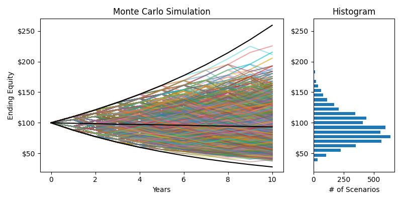
The black lines on the Monte Carlo simulation represent the maximum ($259.40, +259.4%), minimum ($27.90, -72.1%), and mean ($91.30, -8.7%) returns for this stock over 10 years. The actual returns are a random walk, and it could be any of these lines or the 9.695 million lines I didn't show. But look at this histogram. Sure it's a little skewed, but it sure as hell looks like a bell curve. Using Monte Carlo, We've created a representative sample of the population of possible returns. We'll do the same trick from Three Six Mafia to normalize our data by taking the natural log of each data point.
Normalized Histogram of Returns
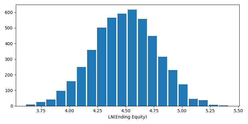
$$\mu = 4.489$$ $$\sigma = 0.2787$$
To illustrate that this normalized data set does a good job of describing the findings from our Monte Carlo simulation, let's check the extreme ends. What values are at the 0.001 percentile and the 99.999 percentile? Don't forget we have to raise e to that value to get back to dollar amounts.
$$Extreme_{x} = e^{NORM.INV(percentile, \mu, \sigma)}$$ $$Extreme_{Low} = e^{NORM.INV(0.00001, 4.489, 0.2787)} = $27.03$$ $$Extreme_{High} = e^{NORM.INV(0.99999, 4.489, 0.2787)} = $251.17$$
That is pretty close to the actual calculated limits of $27.90 and $259.40. Remember statistics is never meant to give you hard numbers. Statistics describes our data, it isn't our data.
Getting Real Petty
The scenario we created for our various Pay it Forward Trains is remarkably similar to the Monte Carlo demo that we just did. In fact we can take the same approach, split it by number of passengers, and track over/under payment instead of investment growth. We'll run our Monte Carlos simulation of getting caught in a PiFT thousands of times, and then produce 7 distributions curves from that simulation.
Because ultimately, we can't be the type of person who just communicates and makes decisions. We need statistical analysis to forecast every scenario in our life and predetermine our response. A totally normal way to live.
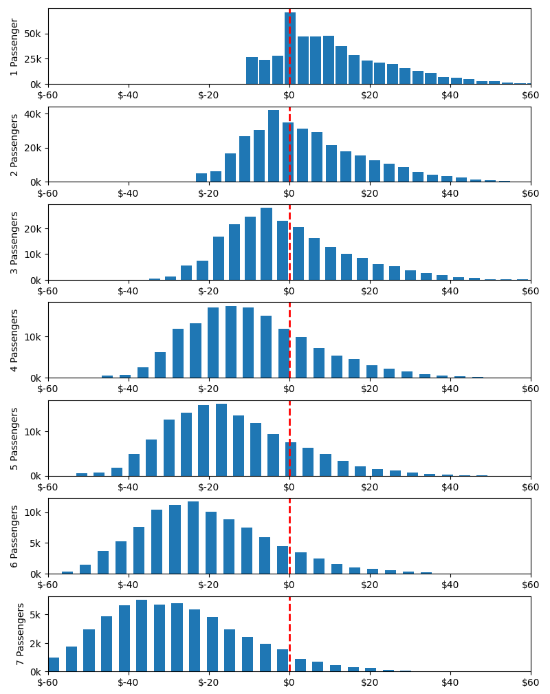
Histograms of Over/Under Payment for Passengers
Violin of Over/Under Payment by Passengers
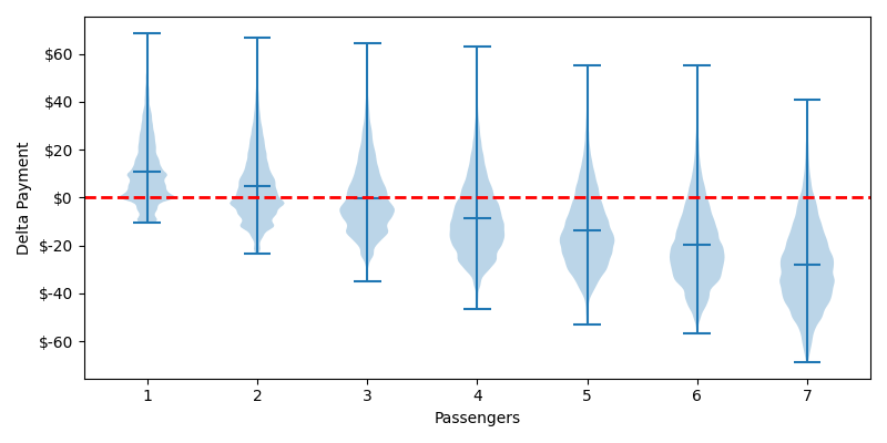
These charts shouldn't shock you. If you can't intuit that an order for 7 passengers is likely to be more expensive than any random car, well I don't know how you're still reading. But now we can answer some pedantic questions down to the decimal point. Before we answer those questions, we need to address some lumpiness in our data. Lumpiness is different than skewness, natural log won't help us.
The lumpiness is most extreme in our single passenger distribution. It gets smaller as the number of passengers grows, but it never fully disappears. However we can think through a few things to understand the source of this lumpiness and even predict where the lumps will occur. To do that, let's look at a histogram of all 1.48 million cars by passenger type.
Histogram of Cars by # of Passengers
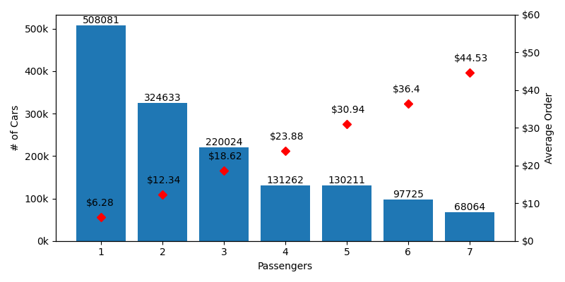
Because of our pseudo-random passenger selection, there are WAY more single passenger cars than any other type. In every scenario, there is a ~1:3 chance that the car behind you is a single passenger car who has the lowest average order of $6.28. If we make a quick table comparing the average order of each number of passengers to the single occupant, you'll see that the difference roughly lines up with our lumpiness.
| # of Passengers | Avg Single Order Total | Avg Order Total | Difference |
|---|---|---|---|
| 1 | $6.28 | $6.28 | $0.00 |
| 2 | $6.28 | $12.34 | -$6.06 |
| 3 | $6.28 | $18.62 | -$12.34 |
| 4 | $6.28 | $23.88 | -$17.60 |
| 5 | $6.28 | $30.94 | -$24.66 |
| 6 | $6.28 | $36.40 | -$30.12 |
| 7 | $6.28 | $44.53 | -$38.25 |
Of course, the other cars play an impact as well. There's a ~1:4 chance the car will be behind you will have 2 passengers and a ~3% chance it will have 7. To fully calculate the location of the lump you would just do a weighted average of the difference between all other cars and their likeliness of being behind you.
$$Lump_{passengers} = \sum_{i=1}^{7} Weight_{i} * (AvgOrder_{i} - AvgOrder_{passengers})$$
What's at Risk Here?
Like the brains of whomever starts a PiFT, our data is a little lumpy. We can still use it though. Our bell curve is a predictive model, it's not the real world. So back to our questions:
How Risky is the PiFT based on number of passengers?
I'm glad you asked. To answer this question we first need to determine your risk tolerance. Let's say you are willing to pay up to 50% more than your original order to avoid the public shaming associated with ending the train. The average order for a single person is $6.28, so you're willing to pay up to $9.42 before common sense prevails. The mean over payment for a single passenger is $10.30 with a stdev of $13.81. Using our Norm.Dist() function we can calculate the probability of paying more than $9.42.
$$ P(Getting\ the\ Shaft) = 1 - NORM.DIST( OverPayment_{Max}, \mu, \sigma, true) $$ $$ P(Getting\ the\ Shaft) = 1 - NORM.DIST( $9.42, $10.30, $13.81, true)$$ $$ P(Getting\ the\ Shaft) = 69.7\%$$
Nice. 69.7% of the time, you'll get screwed every time and have to pay more than 150% of your original order as a single passenger. It's probably best to avoid drive-throughs all together unless you have buddies along for the ride. We can make a quick table to show the odds for all number of passengers that you can print out and stick on your dash:
| # Passengers | 50% Over Payment | μ Over Payment | σ Over Payment | P(Getting the Shaft) |
|---|---|---|---|---|
| 1 | $9.42 | $10.30 | $13.81 | 69.7% |
| 2 | $18.51 | $4.01 | $14.01 | 43.9% |
| 3 | $27.93 | -$2.12 | $14.55 | 21.6% |
| 4 | $35.82 | -$7.67 | $14.64 | 9.0% |
| 5 | $46.41 | -$14.41 | $15.11 | 2.4% |
| 6 | $54.60 | -$22.15 | $16.06 | 0.6% |
| 7 | $66.80 | -$26.10 | $17.12 | 0.2% |
Is there a defensive order amount just in case we get caught in a PiFT?
Is this new-found fear of PiFTs keeping you up with anxiety? Sleepless nights spent tossing and turning while lamenting the fact that you can no longer visit any drive through for risk of being asked to pay more. Don't worry, we can easily use the same data to help you place an order that has a 99.9% chance of guaranteeing that you don't end up overpaying in this event. We'll just use our Norm.Inv() to find out what that order would be for a single person. Except this time, we don't want to look at passenger specific distributions. We need to compare against distributions of all over/under payments which has a mean of $0.00 and stdev of 18.26.
$$ Defensive\ Order = NORM.INV(probability, \mu, \sigma )$$ $$ Defensive\ Order = NORM.INV(0.999, 0.00, $18.26) $$ $$ Defensive\ Order = $56.43$$
So as long as you're willing to order 4 Big Mac Meals with an extra QP w/ C, you can be confident that you won't be the victim of a PiFT. I'll let you calculate the costs associated with gout and buying a new toilet.
55 Burgers, 55 Fries
This entire time we've been operating under the assumption that every party to the Pay it Forward Train is acting in good faith. Sure they're idiots, but idiots blind to the arbitrage opportunity available to them. Let's imagine a rogue actor starts a PiFT in an attempt to circle the building and place an absurdly large order. Say, I don't know, 55 Burgers, 55 Fries, 55 Pizzas, & 55 Pies? McDonalds doesn't sell pizzas, so we'll substitute a 6pc McNuggets.
| Order Item | Price | Qty | Total Price |
|---|---|---|---|
| Quarter Pounder with Cheese | $6.39 | 55 | $351.45 |
| French Fry | $2.49 | 55 | $136.95 |
| 6pc McNuggets | $3.65 | 55 | $200.75 |
| Apple Pie | $2.06 | 55 | $113.30 |
| Total | $802.45 | ||
This monstrosity of an order is well beyond the scope of even what we would from even a cargo van full of ravenous adults. What happens if we randomly insert this order into each of our simulated trains? How does it change the minimum defensive order we would need to place?
Honestly, the charts don't really help us portray the data as our distributions break down. I'll show the Violin chart to show how extreme our distributions are.
I Think you Should Violin
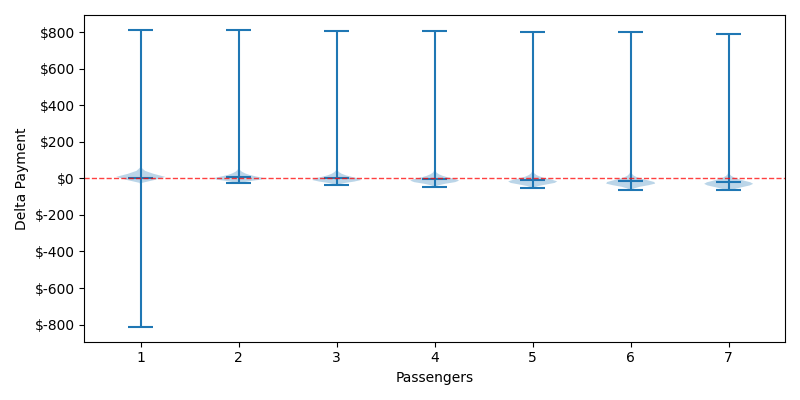
The lower end of our distributions for 2-7 passengers hasn't really changed, but we now have long-tail outlier events where somebody gets caught paying for this $800 order. The single passengers face this same risk, except our rogue actor's free month of groceries is also reflected as a lower long-tail event. To calculate how much our defensive order needs to increase, we'll create a new distribution of all the over/under payments minus for our rogue actor. Our new mean is $5.30 with stdev of $67.14 which means that we need to change our defensive order to $212.78 if we want to have 99.9% confidence that we won't over pay in a PiFT even in this extreme case. The best course of action may be to avoid fast food entirely, or at least call ahead and inquire about their maximum order policy.
ACKHYUALLY...
Now, I intentionally left in a flawed way of thinking here so we can talk about why intuition is such an important part of statistics. Our defensive order increased from $56 to $212 because of the presence of Mr. 55 Burgers. I mentioned that our distributions were breaking down, but we can still easily calculate the mean and stdev and treat it is normalized. However, if we don't look at the shape of our data (i.e. histogram) we'd never see the flaw.
Let's think about how this scenario plays out with the knowledge that there is only one $800 order per train:
| Scenario A Mr. 55 Burgers Is Not Behind You |
Scenario B Mr. 55 Burgers IS Behind You |
|---|---|
| This $800 order has no impact on you. He is the only one aware that the PiFT is happening because he started it. So if he is not behind you, your defensive order shouldn't change at all. | Well now you've created a massive $212 order and placed that burden on the innocent soul in front of you. However, you're still over paying by almost $600 so the defensive order has merely lessened your pain instead of removing it. |
This is why intuition is so important, and why you need to understand the shape of your data. Your defensive order of $56 is completely valid 148/150 or 99% of the time. It's that 1:150 chance where you are asked to pay $800 and your defensive order has failed. My suggestion is to always call ahead and ask about their "maximum order policy". This way you can eliminate outlier events and rely on our previous data model.
If the road to hell is paved with good intentions, PiFT most certainly leads to Dante's ninth circle. Empowered by this critical knowledge, you should have no hesitation if you too are ever asked, "would you like to pay for the car behind you?" Unless, of course, you're one of those people who places a value on things like "being kind".